Number of rays: 12191 (P phases: 7648, S phases:
4543)
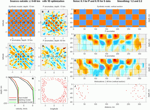
This test is designed to model a case
when all the sources are located outside the network. According to an existing
stereotype, all the events with GAP>180 should be not considered in
local-earthquake tomography, thus no reasonable results can be achieved using
this dataset. At the same time, everybody can check that this is not
true.
In this test, reference 1D velocity model is
presumed to be unknown. The values in "refmod.dat" are not
exact and are estimated using 1D optimization in the LOTOS-07 code. The initial coordinates of the sources in file "rays.dat" correspond to the source locations based on the approximate 1D reference model in "refmod.dat". Configuration of the model, data setup and inversion results obtained using LOTOS-07 code are shown in FIGURE 2:

Figure
2. Inversion results using the sources located outside the network.
A and E:
synthetic model in a horizontal section ( 15
km depth) and vertical section (position of the section
is indicated in A). Triangles show locations of stations.
B,C and D: resulting P velocity anomalies in
horizontal sections. F and G resulting
velocity anomalies of P and S velocities in a vertical section shown in plots
A-D. H: result of the 1D model optimization. Red line is the
true model; black line is the starting model; green line is the retrieved model.
I and J : locations of events in map view and
in the vertical section. Red dots are relocated sources; bars show errors with respect to true coordinates.
The data for this test can be downloaded using this link:
"download inidata.zip" .
Details of this test are given
HERE.
The other examples are BLIND tests without any
information about initial source locations, 1D velocity model and configurations
of synthetic anomalies.
We present four data sets for different regions, various data
amount and the model complexity (ZIP files can be downloaded by clicking of a
link with a region name).
1. Costa-Rica
2.Turkey
3. Toba (N.Sumatra)
3. Chile, offshore area at 21° latitude
In most cases, source/receiver pairs in these datasets correspond to real observation
systems (Costa-Rica, Turkey, Toba areas). In one dataset (Chile) we use synthetic configuration of sources/receivers created for planning a network deployment.
The dataset for each area includes two files.
1. File with station geographical coordinates (stat_ft.dat)
which includes longitude, latitude and elevation which is given in km. Positive value means that the station is below sea level. In the presented synthetic dataset (Chile), all the stations are at 1 km depth below sea level.
-71.12700 -18.63300 1.000000
-71.09300 -19.31700 1.000000
-71.02700 -20.00000 1.000000
-70.97700 -20.66700 1.000000
-70.91000 -21.31700 1.000000
-70.84300 -21.93300 1.000000
-70.71700 -19.63300 1.000000
-70.63300 -20.28300 1.000000
-70.55000 -20.96700 1.000000
-71.80000 -19.63300 1.000000
-71.70000 -20.28300 1.000000
-71.61700 -20.96700 1.000000
2.
File with initial locations of sources and travel times (rays.dat).
In all presented datasets, as in case of real data, neither coordinates, no origin time of sources are given.
Instead the source coordinates, an arbitrary
point (the center if the study area) is given.
The uncertainty of the origin times is modeled by
adding a random bias to all travel times from each source
First line is a description of an event which includes geographical
coordinates: longitude (degree, W-negative), latitude (degrees, S-negative) and
depth (km), and number of recorded phases, NPhase.
After the line of source description,
NPhase
lines follow. First column is phase indicator (1:P, 2:S), second column is number of station according to the list in "stat_ft.dat". Third column is travel time, in second. Below is example for two events from "rays.dat":
-71.00000 -20.50000 0.0 16
1 11 21.44222
2 11 39.99702
1 8 9.970146
2 8 20.13324
1 3 15.76965
2 3 30.17566
1 9 4.323131
2 9 10.35645
1 4 11.41212
2 4 22.64251
1 5 10.41145
1 2 23.83436
1 6 16.14024
1 10 27.48143
1 12 17.56363
1 7 18.78923
-71.00000 -20.50000 0.0 18
1 10 25.25985
2 10 44.08272
1 3 13.64796
2 3 23.97212
1 11 22.29410
2 11 38.93983
1 1 29.96118
2 1 52.22488
1 2 21.23783
2 2 37.11849
1 5 18.25490
2 5 31.93942
1 7 15.38151
2 7 26.97361
1 12 22.55341
2 12 39.39588
1 8 7.015490
1 4 13.06192
Reconstruction results for the Costa-Rica dataset
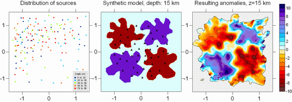
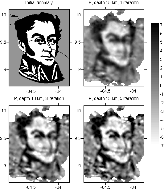
Here we present the results of reconstruction for Costa-Rica dataset, the most complicated test among the four presented datasets. In this test the synthetic anomalies composed the face of Simon Bolivar. The reconstruction based on the same two initial data files, as given in this web site and was performed using LOTOS-07 algorithm . Anybody can repeat the same colculations. To do this, one should download the algorithm EXE version of the code and follow simple instructions on installing and running the programs.
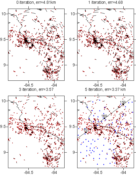
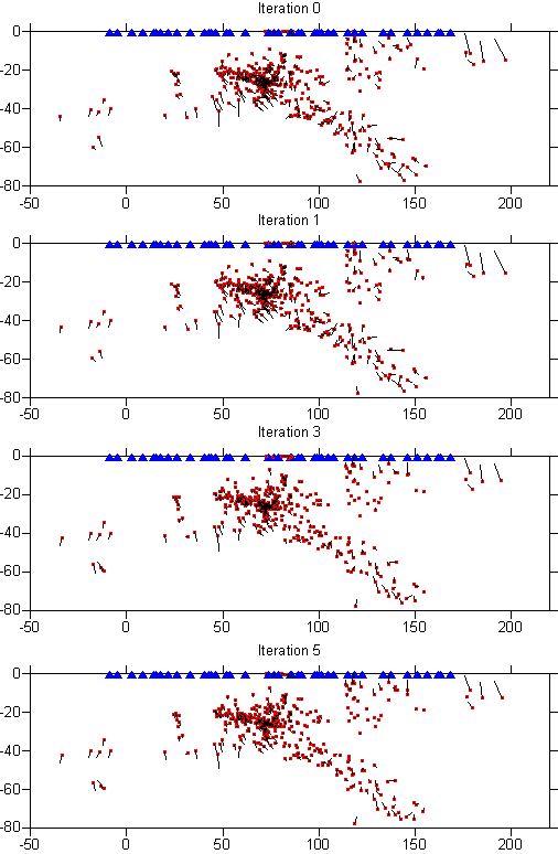
Below we present Figures 3
and 4 with results of source locations in map view and in a cross
section. The starting location for all the sources was at LON= -84.5°, LAT=9.5°
DEPTH=0. Zero iteration means preliminary location in a 1D velocity model using
tabulated travel times. First iteration is a location using 3D ray tracing
(bending) in 1D velocity model. 3 and 5 iterations represent the locations in a
3D models obtained after 2 and 4iterations, respectively.
The results of reconstruction as well as configuration of the initial "true"
model are presented in Figure 5. One can see that the most
reliable results are obtained in 3 iteration. It is amazing that even very thin
patterns like nose contours are visible in the results.
I invite everybody to join this benchmark. I hope to see
the similar results based on my dataset obtained using the other tomographic
codes. I would be interested if anybody produces own datasets to test my
algorithms.

Figure 3. Results
of location in 0, 1, 3 and 5 iterations in the map view. Red dots represent the
current locations. Black bars indicate shifts from "true" locations defined in
the synthetic model. RMS of source location error in indicated in the title of
each map. Location of the cross section indicated in Figure 2 and seismic
stations (blue triangles) are given in the last map.

Figure 4.
Results of location in 0, 1, 3 and 5 iterations in a cross section. Red dots
represent the current locations. Black bars indicate shifts from "true"
locations defined in the synthetic model. Blue triangles show seismic stations
projected to the profile.

Figure 5.
Initial synthetic model and results of reconstruction using LOTOS-07 algorithm after 1, 3 and 5 iterations at the
depth of 15 km.Velocity perturbations are given in percent
